ORSuite Experiment Guide

ORSuite is a collection of environments, agents, and instrumentation, aimed at providing researchers in computer science and operations research reinforcement learning implementation of various problems and models arising in operations research. These experiments are made up of several componets including:

importing packages
specifying the environment
selecting algorithms
running experiment/generating figures

This guide follows the ambulance environment model and will go through how to read and run experiments made by ORSuite.

The ambulance routing problem addresses the problem by modeling an environment where there are ambulances stationed at locations, and calls come in that one of the ambulances must be sent to respond to. The goal of the agent is to minimize both the distance traveled by the ambulances between calls and the distance traveled to respond to a call by optimally choosing the locations to station the ambulances.

For more information on the example see examples/ambulance_metric_environment.ipynb. For more information on the environment see or_suite/envs/ambulance/ambulance_metric.py.

Package Installation

In this section we import the modules required to run experiments within the ORSuite package.

import or_suite # current package used
import numpy as np # open source Python library that aids in scientific computation
import copy # creates a shallow and deep copy of a given object
import os # provides functions for working with operating systems
from stable_baselines3.common.monitor import Monitor #  monitor wrapper for Gym environments, used to know the episode length, time and other data
from stable_baselines3 import PPO # uses clipping so that after an update, the new policy will not be not too far form the old policy
from stable_baselines3.ppo import MlpPolicy # the policy model used in PPO
from stable_baselines3.common.env_util import make_vec_env # stacks multiple different environments into one (vectorized environment)
from stable_baselines3.common.evaluation import evaluate_policy # evaluates the agent and the reward
import pandas as pd # brings pandas data analysis library into current environment

Experimental Parameters

Next we specify the set of parameters for running an experiment. These include both “experiment” parameters and “environment” parameters. The experiment parameters are:

DEFAULT_SETTINGS = {'seed': 1, # allows random numbers to be generated
                    'recFreq': 1, # frequency for saving cumulative H-step rewards per episodes in the dataframe
                    'dirPath': '../data/ambulance/', # a string, is the location where the data files are stored
                    'deBug': False, # prints information to the command line when set true
                    'nEps': nEps, # represents the number of episodes
                    'numIters': numIters, # # the number of iterations of (nEps, epLen) pairs to iterate over with the environment
                    'saveTrajectory': True, # save trajectory for calculating additional metrics
                    'epLen' : 5, # represents the length of each episode
                    'render': False, # renders the algorithm when set to true
                    'pickle': False # indicator for pickling final information
                    }

The experimental parameters can be found in the attributes section of or_suite/experiment/experiment.py.

Environmental specific parameters:

In order to make an environment you type Gym.env('Name', env_config).

The specific configuration of the parameters for each of the environments can be found in or_suite/envs/env_configs.py. In or_suite/envs/env_configs.py, each environment has customizable parameters you can create and set. For the ambulance example the cooresponding parameters are written as:

ambulance_metric_default_config = {'epLen': 5, # number of time steps to run the experiment for
                                   'arrival_dist': lambda x: np.random.beta(5, 2), # the arrival distribution for calls over the space [0,1]
                                   'alpha': 0.25, # controls the proportional difference between the cost to move ambulances in between calls and the cost to move the ambulance to respond to a call
                                   'starting_state': np.array([0.0]), # list containing the starting locations for each ambulance
                                   'num_ambulance': 1, # represents the number of ambulances in the system
                                   'norm': 1 # representing the norm to use to calculate distances; in most cases it should probably be set to 1
                                   }

Agents

The agents section of the code specifies the algorithms used in the experiment. These agents are later ran against each other to see which ones are most effective for the simulation. Each of the agents have different parameters. To check all the agent files in the ambulance example with varying parameters see or_suite/agents/ambulance.

A common agents throughout different experiments is:

Random implements the randomized RL algorithm, which selects an action uniformly at random from the action space. In particular, the algorithm stores an internal copy of the environment’s action space and samples uniformly at random from it.

Other agents are further specified within each experiment in “ORSuite/examples”.

Median is an agent that takes a list of all past call arrivals sorted by arrival location, and partitions it into k quantiles where k is the number of ambulances. The algorithm then selects the middle data point in each quantile as the locations to station the ambulances.

Stable is an agent that only moves ambulances when responding to an incoming call and not in between calls.

SB PPO is Proximal Policy Optimization. This agent comes from stable_baselines_3. When policy is updated, there is a parameter that “clips” each policy update so that action update does not go too far.

AdaQL is an Adaptive Discretization Model-Free Agent, implemented for enviroments with continuous states and actions using the metric induced by the l_inf norm.

AdaMB is an Adaptive Discretizaiton Model-Based Agent, implemented for enviroments with continuous states and actions using the metric induced by the l_inf norm.

Unif QL is an eNet Model-Based Agent, implemented for enviroments with continuous states and actions using the metric induces by the l_inf norm.

Unif MB is a eNet Model-Free Agent, implemented for enviroments with continuous states and actions using the metric induces by the l_inf norm.

Specifying the agents in the code looks like:

agents = { 'SB PPO': PPO(MlpPolicy, mon_env, gamma=1, verbose=0, n_steps=epLen),
'Random': or_suite.agents.rl.random.randomAgent(),
'Stable': or_suite.agents.ambulance.stable.stableAgent(CONFIG['epLen']),
'Median': or_suite.agents.ambulance.median.medianAgent(CONFIG['epLen']),
'AdaQL': or_suite.agents.rl.ada_ql.AdaptiveDiscretizationQL(epLen, scaling_list[0], True, num_ambulance*2),
'AdaMB': or_suite.agents.rl.ada_mb.AdaptiveDiscretizationMB(epLen, scaling_list[0], 0, 2, True, True, num_ambulance, num_ambulance),
'Unif QL': or_suite.agents.rl.enet_ql.eNetQL(action_net, state_net, epLen, scaling_list[0], (num_ambulance,num_ambulance)),
'Unif MB': or_suite.agents.rl.enet_mb.eNetMB(action_net, state_net, epLen, scaling_list[0], (num_ambulance,num_ambulance), 0, False),
}

Running The Code and Generating Figures

There are two types of experiment files:

an sb_experiment file, runs a simulation between an arbitrary openAI Gym environment and a stable baselines algorithm, saving a dataset of (reward, time, space) complexity across each episode, and optionally saves trajectory information. It uses parameters self, env, model, and dict .
a normal experiment file, runs a simulation between an arbitrary openAI Gym environment and an algorithm, saving a dataset of (reward, time, space) complexity across each episode and optionally saves trajectory information. It uses parameters self, env, agent, and dict .

After running the “Running Algorithm” section, the experiment will run and the agents/algorithms will show up in a chart. This chart will show all of the agents running against each other, with their reward, time and space. With this information one can see which agents are ideal for their goal. Some environments like the metric ambulance will also show MRT (mean response time) and RTV (response time variance).

Following the chart, line and radar plots will appear to show how each agent responds visually.

Example:

When running each of the algorithms they all start with empty lists for each of the paths.

path_list_line = []
algo_list_line = []
path_list_radar = []
algo_list_radar = []

Then there is a for loop that loops over the agents. Within this for loop, there are if/elif/else statements to check to see what the current agent at use is. The dirPath parameter allows each environment to follow its own direction and therefore create their own radar and line plots. It allows the algorithms to be represented as distinct paths so that the data files don’t overwrite one another. We store them in a list so that the plots all refer to the correct data files

for agent in agents:
    print(agent)
    DEFAULT_SETTINGS['dirPath'] = '../data/ambulance_metric_'+str(agent)+'_'+str(num_ambulance)+'_'+str(alpha)+'_'+str(arrival_dist.__name__)+'/
    if agent == 'SB PPO':
        or_suite.utils.run_single_sb_algo(mon_env, agents[agent], DEFAULT_SETTINGS)
    elif agent == 'AdaQL' or agent == 'Unif QL' or agent == 'AdaMB' or agent == 'Unif MB':
        or_suite.utils.run_single_algo_tune(ambulance_env, agents[agent], scaling_list, DEFAULT_SETTINGS)
    else:
        or_suite.utils.run_single_algo(ambulance_env, agents[agent], DEFAULT_SETTINGS)

    path_list_line.append('../data/ambulance_metric_'+str(agent)+'_'+str(num_ambulance)+'_'+str(alpha)+'_'+str(arrival_dist.__name__))
    algo_list_line.append(str(agent))
    if agent != 'SB PPO':
        path_list_radar.append('../data/ambulance_metric_'+str(agent)+'_'+str(num_ambulance)+'_'+str(alpha)+'_'+str(arrival_dist.__name__))
        algo_list_radar.append(str(agent))

Additional metrics (like MRT and RVT) can be added in or_suite/utils.py:

def mean_response_time(traj, dist):
    mrt = 0
    for i in range(len(traj)):
        cur_data = traj[i]
        mrt += (-1) * \
            np.min(
                dist(np.array(cur_data['action']), cur_data['info']['arrival']))
    return mrt / len(traj)

Then, the additional metrics are called by using the definition made earlier, and inserting the parameters traj, lambda, x and y. To insert the additional metrics in the figure, fig_name is redefined with additional_metric inserted as a parameter for or_suite.plots.plot_radar_plots.

additional_metric = {'MRT': lambda traj : or_suite.utils.mean_response_time(traj, lambda x, y : np.abs(x-y)), 'RTV': lambda traj : or_suite.utils.response_time_variance(traj, lambda x, y : np.abs(x-y))}

fig_name = 'ambulance_metric'+'_'+str(num_ambulance)+'_'+str(alpha)+'_'+str(arrival_dist.__name__)+'_radar_plot'+'.pdf'
or_suite.plots.plot_radar_plots(path_list_radar, algo_list_radar,
fig_path, fig_name,
additional_metric)

Afterwards, a table of agents with each of their rewards, time, space, and for some environments MRT and RTV appears. An example of this table is:

  Algorithm    Reward      Time    Space       MRT       RTV
  Random -1.671218  6.935870 -5053.90 -0.326093 -0.050874
  Stable -1.032668  7.530278 -4283.30 -0.285655 -0.064205
  Median -0.875958  6.638060 -5044.62 -0.212675 -0.043899
   AdaQL -1.113290  6.449667 -4905.76 -0.265052 -0.041170
   AdaMB -1.113290  6.590761 -4596.32 -0.265052 -0.041170
 Unif QL -2.137630  6.591951 -4620.32 -0.430012 -0.089006
 Unif MB -2.299622  6.210666 -4620.32 -0.454634 -0.091324

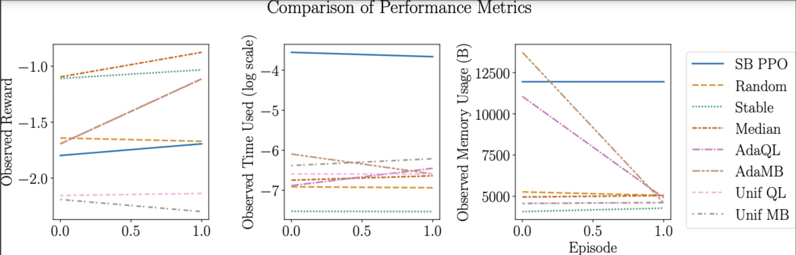
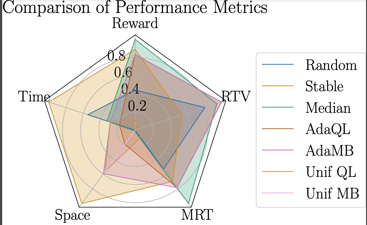
Once the algorithms are run, the figures are created. Each of the environments will create three line plots and one radar plot to show how the difference in agents.

Radar Plot

The radar plot below shows the agents (color coded in the box on the right) with the variables the agents are tested against on each end of the radar plot. The larger the surface area covered by the plot, the better the algorithm performs across a wider range of metrics.

figureRadarPlot = 'ambulance_metric'+'_'+str(num_ambulance)+'_'+str(alpha)+'_'+str(arrival_dist.__name__)+'_radar_plot'+'.pdf'
IFrame("../figures/" + figureRadarPlot, width=600, height=450)

Line Plot

The line plots also have all of the agents color coded in a box on the right. The first plot shows the reward of each agent. The second one shows the obersved time used on a log scale, and the third shows the observed memory usage (B).
Here is an example of how to write the code for a line plot.

from IPython.display import IFrame
figureLinePlot = 'ambulance_metric'+'_'+str(num_ambulance)+'_'+str(alpha)+'_'+str(arrival_dist.__name__)+'_line_plot'+'.pdf'
IFrame("../figures/" + figureLinePlot, width=600, height=280)