import numpy as np
import matplotlib.pyplot as plt
from dynamics_model_4groups import dynamics_model
The Vaccine Allocation Problem
Description
Given a limited number of available vaccines and a population undergoing an epidemic, how do we distribute vaccines to the population in a way that achieves some goal (like minimizing death or maximizing the potential for herd immunity)? The vaccine allocation or allotment problem considers the question: If we divide the population into different groups or risk classes, is there an optimal way to allocate the vaccines across these groups so that we minimize infections, deaths or hospitalizations? We approach this problem from a reinforcement learning perspective.
4 Groups with Finite Action and Finite State Spaces
The file vacc_4groups.py contains an implemenation of an RL
environment for the vaccine allotment problem with 4 possible risk
groups, a finite action space, and a finite state space. In this
problem, we consider a scenario where the agent chooses a priority
order of the 4 risk groups. This means that vaccines are allocated in a
particular order until there are no more vaccines. In other words,
vaccines are given to eligbile recipients of priority group #1 until
there are no eligible recipients left or the vaccine supply is
exhausted. If there are vaccines left after all eligible people priority
group #1 are vaccinated, then priority group #2 can be vaccinated and so
on.
Reinforcement Learning Problem Setup
Markov Decision Process (MDP)
At each time step \(t\) in the RL environement, we have a population of size \(P\) split into four classes \(C_1^t, C_2^t, C_3^t\) and \(C_4^t\). Here, \(C_i^t\) denotes the size of class \(i\) at time \(t\).
We further split each class \(C_i\) into two groups: susceptbile \((S_i^t)\) and asymptomatically infected \((A_i^t)\). We keep track of the aggregate totals of symptomatically infected individuals, both mild (\(I^t\)) and requiring hospitalization (\(H^t\)).
For each time period \(t\), we also keep track of new infections that have occurred since time step \(t-1\). We define this as
In other words, we take the total number of infections at time \(t\) and subtract the total number of infections from time \(t-1\) to determine how many infections are new.
We form the MDP \((\mathcal{S}, \mathcal{A}, \mathcal{T}, \mathcal{R})\) where + The state space \(\mathcal{S}\) is defined as \(\mathcal{S} := [P]^{11}\) with \([P] := \{0, 1, 2, \ldots, P\}\). Recall that \(P\) is the total population size. Each tuple in the space is of the form
and thus tells us how many people are suceptible, infected and to which group they belong (if applicable) at time step \(t\). + The action space is defined by
where a permuation of \(\{1,2,3,4\}\) defines a priority order of the 4 classes and an empty list defines “no priority order,” aka random vaccination. + The transition dynamics \(\mathcal{T}\) are given by the transitions in the continuous time Markov chain (CTMC) specified below. > The state space of the CTMC is almost exactly the same as the MDP. The state space in this case is also \([P]^{11}\), but in this case a state at a time \(t\) is of the form
The difference being that instead of the \(N^t\) term in the state space of the MDP, we have an \(R^t\) term, where \(R^t\) denotes the number of recovered individuals at a given time \(t\). Recovered individuals include anyone who has been vaccinated and anyone who has recovered from infection. > > The initial state \((S_1^0, S_2^0, S_3^0, S_4^0, A_1^0, A_2^0, A_3^0, A_4^0, I^0, H^0, R^0)\) is specified as an initial condition by the user. > > All events in this CTMC are implemented as independent Poisson processes. For example, the times between meetings for all the groups (i.e. an interaction between group \(i\) and group \(j\)) are given by Poisson processes with rates specified by the user. In this case, we must specify a \(4 \times 4\) contact matrix \(\Lambda\) where the \((i,j)\)th component corresponds to the meeting rate between the \(i\)th and \(j\)th groups. > > Only infectious meetings are calculated, meaning we only keep track of meetings between infected individuals and susceptible individuals. Each rate is a rate between two people, so we have to scale the meeting rates by the number of people in each class. This means that the rates change over time. Once a person in class \(i\) has been infected, they have probability \(p_i\) of developing symptoms. If a person in class \(i\) develops symptoms, they have probability \(h_i\) of those symptoms requiring hospitalization. > > There is also a recovery rate \(\beta\) and a vaccination rate \(\gamma\). The vaccination rate corresponds to the average number of people that can be vaccinated per day and remains constant. However, the recovery rate is scaled by the number of people who are infected and thus changes over time. > > Each individual Poisson process has an associated exponetial random variable “clock” with the same rate as the Poisson process. This gives us a collection of exponential timers. The minimum of several independent exponential random variables is also an exponential random variable, but with a rate equal to the sum of all the rates of the independent exponential random variables. Therefore, to calculate the time of the next event, we sum up the meeting, recovery, and vaccination rates and pass this sum as the rate of an exponential random variable.
The reward (or cost, in this case) \(\mathcal{R}\) recieved after transitioning from state \(s\) to state \(s'\) due to an action \(a\) is equal to negative one times the total number of infections in state \(s'\) minus the total number of infections at state \(s\), aka the new infections that occurred during this transition. If \(s = s_{t-1}\) is the state at time \(t-1\) and \(s' = s'_t\) is the state at time \(t\), then \(\mathcal{R}_a(s,s') = -N^t\).
Model Assumptions The total population is kept constant throughout the entire time horizon. There are precisely 4 risk classes, with the first class corresponding to medical workers. Vaccines are administered by priority group. The first priority group is vaccinated until there are either no more eligible vaccination candidates or there are no more vaccines. If vaccines remain, the next priority group is vaccinated and so on. Asymptomatic individuals are never vaccinated. >For details about the assumptions made in implementing the SIR disease dynamics model, please refer to the section titled Disease Dynamics below.
State Space
The state space for this environment is discrete, consisting of tuples of integer values representing certain population stats. > In this case, an element of the state space looks like
where > + \(P =\) the total population size > + \(S_1,S_2,S_3,S_4 =\) the total # of susceptible people in groups 1, 2, 3 and 4, resp > + \(A_1,A_2,A_3,A_4 =\) the total # of asymptomatically infected people in groups 1, 2, 3 and 4, resp > + \(I =\) total # of mild symptomatic infections > + \(H =\) total # of hospitalized infections and > + \(N =\) total # of NEW infections (includes asymptomatic and symptomatic) that occurred.
Action Space
The action space for this environment is finite, consisting of 25
possible actions. An action in this space is choosing a priority order.
A valid priority order is either (1) no priority order, aka vaccinate
susceptible people in the population randomly, or (2) a permuation of
\(\{1, 2, 3, 4\}\). > This is represented in vacc_4groups.py as
\(A =\{0, 1, 2, ..., 24\}\), where each number maps to a particular
action. In the file, an action is represented by a number
\(i \in A\) where the corresponding action is at index \(i\) of
the list all_priority_orders. 0 corresponds to [], which means
no priority order. The list is below:
all_priority_orders = [[], ["c1","c2","c3","c4"],["c2","c1","c3","c4"],["c3","c1","c2","c4"],["c1","c3","c2","c4"], ["c2","c3","c1","c4"],["c3","c2","c1","c4"],["c4","c2","c1","c3"],["c2","c4","c1","c3"], ["c1","c4","c2","c3"],["c4","c1","c2","c3"],["c2","c1","c4","c3"],["c1","c2","c4","c3"],["c1","c3","c4","c2"],["c3","c1","c4","c2"],["c4","c1","c3","c2"],["c1","c4","c3","c2"],["c3","c4","c1","c2"],["c4","c3","c1","c2"],["c4","c3","c2","c1"],["c3","c4","c2","c1"],["c2","c4","c3","c1"],["c4","c2","c3","c1"],["c3","c2","c4","c1"],["c2","c3","c4","c1"]]
Reward
The reward, or cost, is precisely equal to (negative) the number of new infections that occurred in this step. By maximizing this quantity, we minimize the number of new infections.
Transitions
Transistions between states are governed by the disease dynamics
implemented in dynamics_model_4groups.py file and described below
under the section Disease Dynamics. In short, the current state and
action are fed to the function dynamics_model imported from the
aforementioned file. This function then returns the new state as well as
some additional information that can be used to plot the population
dynamics.
Environment
The following functions are part of the RL environment implentation
found in the file vacc_4groups.py. > init initializes an
instance of the VaccineEnvironment class; takes in a parameter
config, a dictionary of values used for different purposes
throughout the environment. The dictionary config should contain the
following keys and corresponding values: > + 'eplen': number of time
steps > + 'starting_state': np.array of initial population group
sizes, in the order described above under the State Space section.
Note that at index 10 we have \(N\), the number of new infections in
this time period. This should be set to 0 since new infections are
defined by the current state and a previous state. When we initialize,
there is no previous state. > + 'parameters': dictionary of
parameter values to pass to dynamics model including information such as
contact rates, length of a time step (in days), starting priority order,
etc. More information about these can be found in the section titled
Disease Dynamics below, under the subsection How to use
``dynamics_model_4groups.py``.
 parameters = {'contact_matrix': np.array([[0.0001, 0.0001, 0.00003, 0.00003, 0, 0.0001], [0, 0.0001, 0.00005, 0.0001, 0, 0], [0, 0, 0.00003, 0.00003, 0, 0], [0, 0, 0, 0.00003, 0, 0]]), 'P': np.array([0.15, 0.15, 0.7, 0.2]), 'H': np.array([0.2, 0.2, 0.8, 0.3]), 'beta': 1/7, 'gamma': 100, 'vaccines': 500, 'priority': ["1", "2", "3", "4"], 'time_step': 7}

 initial_conditions = np.array([1990, 1990, 1990, 1990, 10, 10, 10, 10, 0, 0, 0])

 # example of what the config dictionary should look like
 config = {'epLen': 6, 'starting_state': initial_conditions, 'parameters': parameters}


``reset`` returns the environment to its original state

``step(action)`` takes an action from the agent and returns the state
of the system after this action is taken + action: an integer between
0 and 24 corresponding to the index of the ``all_priority_orders``
list that corresponds to the chosen priority order; i.e. the action
is found via ``all_priority_orders[action]`` > + e.g. “no priority
order” would be action :math:`=0`, since
``all_priority_orders[0] = "[]"`` > +
e.g. “:math:`C_1, C_2, C_3, C_4`” would be action :math:`=1` since
``all_priority_orders[1] = ["c1","c2","c3","c4"]"``

The function ``step(action)`` returns + ``newState``: np.array of
integers representing the new state (see state space description
above) + ``reward``: integer value equal to the number of new
infections that occurred in this step and multiplied by :math:`-1` +
``done``: either 0 or 1; flag for the end of the episode + ``info``:
dictionary of information we can use to plot ``disease`` dynamics for
this step

``render`` is currently unimplemented

``close`` is currently unimplemented
Disease Dynamics
Consider a population of \(P\) individuals split into four risk classes: medical workers (\(C_1\)), non-medical essential workers (\(C_2\)), high risk individuals (\(C_3\)) and everyone else (\(C_4\)). Each risk class is further subdivided into five groups: 1. susceptible to the disease (but not infected) 2. asymptomatically infected 3. infected with mild symptoms, 4. infected with severe symptoms (assumed to require hospitalization) 5. recovered or vaccinated or otherwise immune
We keep track of the susceptible people in each class \((S_i)\) and the asymptomatically infected individuals in each class \((A_i)\). However, we only keep aggregate totals of people infected with mild symptoms \((I)\), people who are hospitalized \((H)\) and those who have recovered \((R)\).
Assumptions
In forming the SIR compartmental model, we have made the following assumptions. 1. There are no births, deaths or immigration. 2. People who are infected with mild symptoms perfectly quarantine, and hence do no interact with others in the population. 3. People who are infected with severe symptoms are hospitalized and only interact with medical workers. 4. Vaccines are only administered to susceptible individuals (i.e. infected or recovered individuals are ineligible). 5. Recovery is permanent, i.e. once someone has recovered from infection they are immune to infection.
Model Details/Approach
The model is implemented as a continuous time Markov chain, where events such as infection, recovery and vaccination are modeled as independent Poisson processes. > Contact, or meeting, rates within and between classes are defined by a \(4 \times 4\) matrix, where the \((i,j)\)th entry is the contact rate between class \(i\) and class \(j\). We only account for infectious meetings, by which we mean that when an infected person “contacts” a susceptible person, the susceptible person will get infected. Hence, the contact rate is really the rate of contact AND infection. Also, these meeting rates are the rate between two people and hence must be scaled by the total number of people in each group. As a consequence, these rates change over time. > > People from class \(i\) who are infected have probability \(p_i\) of that infection being symptomatic. If someone in class \(i\) is symptomatically infected, they have probability \(h_i\) of the symptoms being severe and thus requiring hospitalization. > > The recovery rate \(\beta\) is also scaled by the number of people that are infected and hence changes over time. > The vaccination rate \(\gamma\) remains constant since the number of available vaccines does not depend on the state of the Markov chain.
Note that the contact matrix \(\Lambda\), the probabilities \(p_i\) and \(h_i\) for \(i=1,2,3,4\), the recovery rate \(\beta\), and the vaccination rate must all be specified by the user.
How to use the ``dynamics_model_4groups.py`` file
There are three functions inside this file, but the only one the user
ever needs to call is dynamics_model, which takes the following
inputs: a dictionary called parameters and a numpy array called
population.
Input: a dictionary containing the following key and values >
'contact_matrix': (np.array) contact rates matrix between
asymptomatic and susceptible people in classes (avg per day); should
have shape=() > > P: (np.array) \([p_1, p_2, p_3, p_4]\)
probabilities of becoming symptomatic if infected for classes 1, 2, 3,
and 4, resp. > > H: (np.array) \([h_1, h_2, h_3, h_4]\)
probabilities of being hospitalized if symptomatic for each class > >
'gamma': (float) vaccination rate (average number of vaccines you
can administer per day) > > 'beta': (float) recovery rate (per day)
> > 'priority_order': list representing the priority order > >
'vaccines': number of available vaccines (for one entire step in the
RL environment) > > 'time_step': number of DAYS you want the
simulation to run (if time_step < 0, runs until disease-free state) > >
This is different from the the number of steps in the RL environment.
When you call dynamics_model, it will run for however many “days”
you specify. So, for example, if one step in the environment translates
to taking an action, seeing what happens for one week and collecting the
reward at the end of the week, time_step would be set to 7. Then,
every step in the RL environment corresponds to one week in the disease
dynamics simulation.
Input: a numpy array of population group sizes > at index 0: the current number of susceptible people in group 1 \((S_1)\) > > at index 1: the current number of susceptible people in group 2 \((S_2)\) > > at index 2: the current number of susceptible people in group 3 \((S_3)\) > > at index 3: the current number of susceptible people in group 4 \((S_4)\) > > at index 4: the current number of asymptomatically infected people in group 1 \((A_1)\) > > at index 5: the current number of asymptomatically infected people in group 2 \((A_2)\) > > at index 6: the current number of asymptomatically infected people in group 3 \((A_3)\) > > at index 7: the current number of asymptomatically infected people in group 4 \((A_4)\) > > at index 8: the total number of people who are symptomatic with mild symptoms \((I)\) > > at index 9: the total number of people who are symptomatic with severe symptoms \((H)\) > > at index 10: 0, technically a placeholder. Below are examples of both these inputs.
parameters = {'contact_matrix': np.array([[0.0001, 0.0001, 0.00003, 0.00003, 0, 0.0001], [0, 0.0001, 0.00005, 0.0001, 0, 0], [0, 0, 0.00003, 0.00003, 0, 0], [0, 0, 0, 0.00003, 0, 0]]), 'P': np.array([0.15, 0.15, 0.7, 0.2]), 'H': np.array([0.2, 0.2, 0.8, 0.3]), 'beta': 1/7, 'gamma': 100, 'vaccines': 500, 'priority': ["1", "2", "3", "4"], 'time_step': 2}
population = np.array([1990, 1990, 1990, 1990, 10, 10, 10, 10, 0, 0,0])
The function dynamics_model outputs the (new) RL state at the end of
the simulation and some additional information that can be used to plot
the population dynamics that occurred in this step.
Output: newState is a numpy array with updated population
counts; > For information about what is in each index, look at the
description of the input population above. The only difference is
that now index 10 holds important information: the number of infections
that occurred during the simulation, aka “new infections” \((N)\).
Output: output_dictionary is a dictionary with the following
keys (and values) that can be used to create plots of the disease
dynamics that occurred in this simulation > 'clock times': array of
clock times over simulation > > 'c1 asymptomatic': array of class 1
asymptomatic people for each clock time > > 'c2 asymptomatic': array
of class 2 asymptomatic people for each clock time > >
'c3 asymptomatic': array of class 3 asymptomatic people for each
clock time > > 'c4 asymptomatic': array of class 4 asymptomatic
people for each clock time > > 'mild symptomatic array': array of
aggregate mild symptomatic infections for each clock time > >
'hospitalized array': array of aggregate hospitalized infections for
each clock time > > 'c1 susceptible': array of class 1 susceptible
people for each clock time > > 'c2 susceptible': array of class 2
susceptible people for each clock time > > 'c3 susceptible': array
of class 3 susceptible people for each clock time > >
'c4 susceptible': array of class 4 susceptible people for each clock
time > > 'recovered': array of aggregate recovered people for each
clock time (will include symptomatic but not hospitalized) > >
'total infected': total # of people infected by the end of the
simulation (includes people that were already infected) > >
'total hospitalized': total # of people hospitalized throughout
simualation (includes people that were already hospitalized) > >
'vaccines': # of vaccines left
# example of a call to this function
newState, info = dynamics_model(parameters, population)
We've reached vaccination event number 0.0
We've reached vaccination event number 100.0
# example of the output newState
newState
array([1766, 1980, 1989, 1989, 27, 13, 6, 5, 1, 1, 36])
# example of the keys in the output info
print(info.keys())
dict_keys(['clock times', 'c1 asymptomatic', 'c2 asymptomatic', 'c3 asymptomatic', 'c4 asymptomatic', 'mild symptomatic', 'hospitalized', 'c1 susceptible', 'c2 susceptible', 'c3 susceptible', 'c4 susceptible', 'recovered', 'total infected', 'total hospitalized', 'total recovered', 'vaccines', 'event counts'])
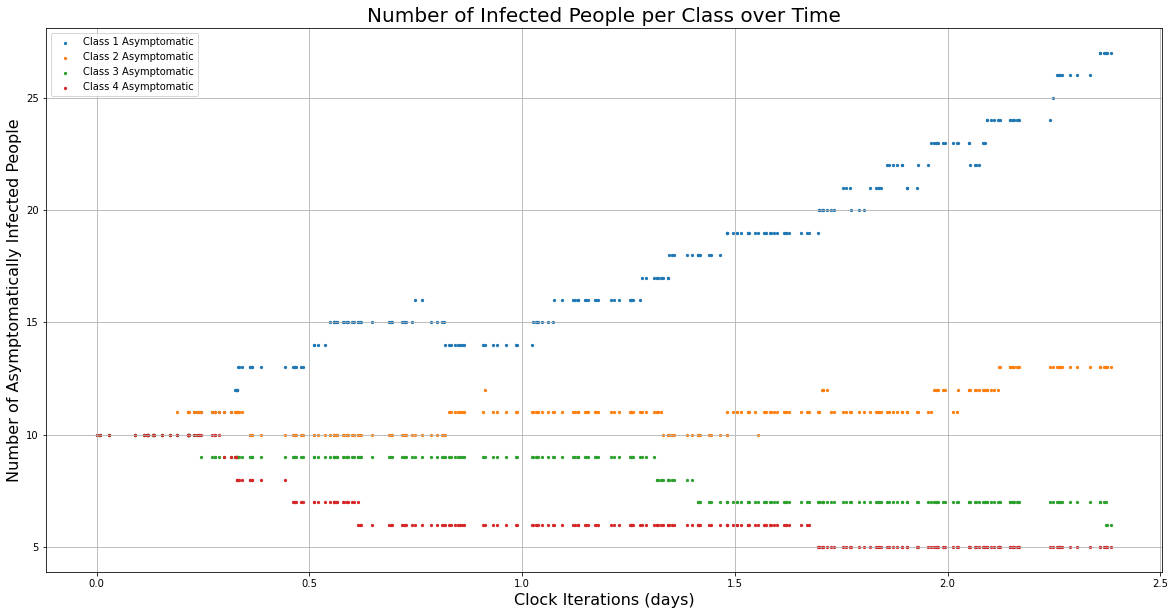
# example of what you can plot using the info dictionary
# adapted from code by Cornell University students Mohammad Kamil (mk848), Carrie Rucker (cmr284), Jacob Shusko (jws383), Kevin Van Vorst (kpv23)

clocks = info['clock times']
c1_A = info['c1 asymptomatic']
c2_A = info['c2 asymptomatic']
c3_A = info['c3 asymptomatic']
c4_A = info['c4 asymptomatic']

figsizex = 20
figsizey = 10
xlabelsize = 16
ylabelsize = xlabelsize
titlesize = 20

%matplotlib inline

fig = plt.figure(figsize=(figsizex,figsizey))
ax1 = fig.add_subplot(111)

ax1.scatter(clocks, c1_A, s=5, marker="o", label='Class 1 Asymptomatic')
ax1.scatter(clocks, c2_A, s=5, marker="o", label='Class 2 Asymptomatic')
ax1.scatter(clocks, c3_A, s=5, marker="o", label='Class 3 Asymptomatic')
ax1.scatter(clocks, c4_A, s=5, marker="o", label='Class 4 Asymptomatic')
plt.legend(loc='upper left');
plt.ylabel('Number of Asymptomatically Infected People',size=ylabelsize)
plt.xlabel('Clock Iterations (days)',size=xlabelsize)
plt.title("Number of Infected People per Class over Time",size=titlesize)
plt.grid(True)
plt.show()
Heuristic Agents
We currently have a single heuristic agent implemented. This algorithm picks a fixed priority order over the different classes and allocates according to that priority order.